
GitHub Repository Link: https://github.com/chinmayp995/CS203-Assignment-7 (All the Python codes are being given in Team 20_Assignment7.ipynb)
Although all the steps play their important role in the assignment; these were the most crucial steps which are also the evaluation criterion for the assignment.
We trained our model using the BOW implementation and we stored our model data in the checkpoint.pt which we then compressed to checkpoint.pt.gz. We saved our checkpoint using torch.save() and when we started the training of the model for IMDB dataset we called this checkpoint which had its best accuracy on its second epoch; we put a try-except statement there which would verify the loading of checkpoint and if there is some error we will be notified. The code for the same goes like
def train_on_imdb(model, imdb_train_loader, imdb_val_loader, epochs=10, checkpoint_path='checkpoint_imdb.pt.gz', resume_checkpoint='checkpoint.pt.gz'):

    writer = SummaryWriter(log_dir='runs/imdb') # starting writer

    #loading model to device and defining optimizers
    model.to(device)
    optimizer = optim.Adam(model.parameters(), lr=0.0001)
    criterion = nn.CrossEntropyLoss()

    imdb_train_losses = []
    imdb_val_losses = []
    imdb_val_accuracies = []
    # load checkpoint if it is  available
    try:
        with gzip.open(resume_checkpoint, 'rb') as f: # decompressing the checkpt
          checkpoint = torch.load(f,map_location=device)
		#loading the state from the checkpt
        model.load_state_dict(checkpoint['model_state_dict'])
        optimizer.load_state_dict(checkpoint['optimizer_state_dict'])
        print(f"Checkpoint loaded! Resuming from this checkpoint")

    except FileNotFoundError:
        print("no checkpoint found, starting training from scratch.")
    #starting to train from start
    start_epoch = 0
    # rest of the code
We see that since we got the best accuracy at the second epoch of the first training we are able to use the model state and the optimizer state from the checkpoints dictionaries and then we start the model training for the embeddings parallelly; And we get excellent accuracies as compared to the earlier training.
This Embedder class initializes an embedding model, first attempting to load Llama-2-7b, but falling back to bert-base-uncased if there are GPU constraints. It tokenizes input text, processes it through the model, and extracts embeddings by averaging the last hidden state. The get_embeddings method returns these embeddings for given texts, ensuring efficient text representation.
#setting up the Embedder class for the LLAma Model
class Embedder:
    def __init__(self):
        try:
            # we try using Llama2-7b which is the latest model; but incase that is not possible we get switch to bert base uncased
            self.tokenizer = AutoTokenizer.from_pretrained("meta-llama/Llama-2-7b")
            self.model = AutoModel.from_pretrained("meta-llama/Llama-2-7b").to(device)
        except Exception:
            print("switch to bert-base-uncased due to GPU constraints.")
            self.tokenizer = AutoTokenizer.from_pretrained("bert-base-uncased")
            self.model = AutoModel.from_pretrained("bert-base-uncased").to(device)

        self.embedding_size = self.model.config.hidden_size
        self.tokenizer.pad_token = self.tokenizer.eos_token
        self.model_loaded = True

    #this helps to get the embeddings
    def get_embeddings(self, texts):
        inputs = self.tokenizer(texts, return_tensors="pt", padding=True, truncation=True, max_length=32).to(device)
        with torch.no_grad():
            outputs = self.model(**inputs)
return outputs.last_hidden_state.mean(dim=1)For getting the parameters logged into the TensorBoard ; we initialised a writer which logs the paramters into the dashboard. The pseudocode goes like
 writer = SummaryWriter(log_dir='runs/imdb') # starting writer

#part of code bla bla bla

#writing the required scalars (n for loop)
writer.add_scalar('IMDB/Train_Loss', avg_train_loss, epoch)
writer.add_scalar('IMDB/Val_Loss', avg_val_loss, epoch)
writer.add_scalar('IMDB/Val_Accuracy', val_accuracy, epoch)

 # logging model parameters
for name, param in model.named_parameters():
      writer.add_histogram(f"IMDB/Params/{name}", param, epoch)


#closing write
writer.close()We load the checkpoint using the torch.load()
def load_checkpoint(model, checkpoint_path='checkpoint.pt'):
    checkpoint = torch.load(checkpoint_path, map_location=device)
    model.load_state_dict(checkpoint['model_state_dict'])
    model.to(device)
    print("Checkpoint loaded successfully.")
However, since the checkpoint can require large amount of memory; We compress that checkpoint to checkpoint.pt.gz which zips that checkpoint. We use shutil and gzip librarries for the same.
def compress_checkpoint(checkpoint_path, compressed_path):
    with open(checkpoint_path, 'rb') as f_in:
        with gzip.open(compressed_path, 'wb') as f_out:
            shutil.copyfileobj(f_in, f_out)
    print(f"Checkpoint compressed and saved as {compressed_path}")
compress_checkpoint('checkpoint.pt', 'checkpoint.pt.gz')For TensorBoard Implementation; we already gave the writers which will log the metrics during the training of the model. Then to get the dashboard for the same we run the following command
%load_ext tensorboard
%tensorboard --logdir runs
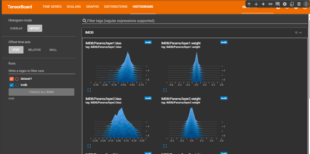
Then we get the dashboard on google collab itselves like this
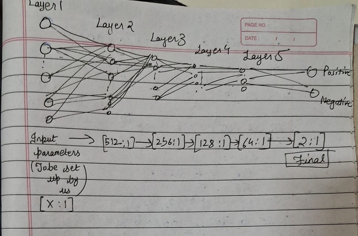
In this assignment we had to use two MLP Models; one for the Bag of Words (BOW) Architecture and other for the Embeddings one. The Model Codes and their configurations are being described below. In the Bag of Words we have used 10k input features such that we get good connections amongst the tokens of the sentences and train well. However, it increases the computational cost and since LLama-3 has 4096 embeddings and it works well for this number of input features (as specified in their documentation) we have used 4096 features for the first layer of MLP Model 2. We have tried using 10k features for MLP2 however that resulted to the crashing of our colab session; So we decided to reduce it. For better aaccuracy we used ReLU Activation and the DropOut Rate of 0.3 at every step.
class MLPModel(nn.Module):
    def __init__(self, input_layer=10000):
        super(MLPModel, self).__init__()
        self.layer1 = nn.Linear(input_layer, 512)
        self.layer2 = nn.Linear(512, 256)
        self.layer3 = nn.Linear(256, 128)
        self.layer4 = nn.Linear(128, 64)
        self.layer5 = nn.Linear(64, 2)
        self.activation = nn.ReLU()
		self.dropout = nn.Dropout(p=0.3)

	def forward(self, x):
        x = self.dropout(self.activation(self.layer1(x)))
        x = self.dropout(self.activation(self.layer2(x)))
        x = self.dropout(self.activation(self.layer3(x)))
        x = self.dropout(self.activation(self.layer4(x)))
        x = self.layer5(x)
        return x
The Model Config outputed as
BOW Model Architecture: MLPModel( (layer1): Linear(in_features=10000, out_features=512, bias=True) (layer2): Linear(in_features=512, out_features=256, bias=True) (layer3): Linear(in_features=256, out_features=128, bias=True) (layer4): Linear(in_features=128, out_features=64, bias=True) (layer5): Linear(in_features=64, out_features=2, bias=True) (activation): ReLU() (dropout): Dropout(p=0.3, inplace=False) ) BOW Model has 5293122 trainable parameters.
class MLP2(nn.Module):
    def __init__(self, input_layer=4096):
        super(MLP2, self).__init__()
        self.layer1 = nn.Linear(input_layer, 512)
        self.layer2 = nn.Linear(512, 256)
        self.layer3 = nn.Linear(256, 128)
        self.layer4 = nn.Linear(128, 64)
        self.layer5 = nn.Linear(64, 2)
        self.activation = nn.ReLU()
        self.dropout = nn.Dropout(p=0.3)

    def forward(self, x):
        x = self.dropout(self.activation(self.layer1(x)))
        x = self.dropout(self.activation(self.layer2(x)))
        x = self.dropout(self.activation(self.layer3(x)))
        x = self.dropout(self.activation(self.layer4(x)))
        x = self.layer5(x)
        return x
Output
Embedding Model Architecture: MLP2( (layer1): Linear(in_features=4096, out_features=512, bias=True) (layer2): Linear(in_features=512, out_features=256, bias=True) (layer3): Linear(in_features=256, out_features=128, bias=True) (layer4): Linear(in_features=128, out_features=64, bias=True) (layer5): Linear(in_features=64, out_features=2, bias=True) (activation): ReLU() (dropout): Dropout(p=0.3, inplace=False) ) Embedding Model has 2270274 trainable parameters.
This diagram is self explanatory regarding the model architecture
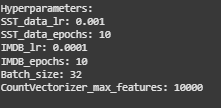
The following are the Hyperparameters we used for both the trainings. Here SST stands for Stanford Sentiment TreeBank which is the initial data we had used for training of BOW Implementation. Also, IMDB dataset was used for the next model after defining the Checkpoint
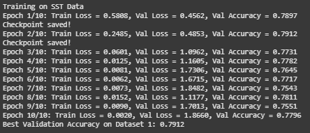
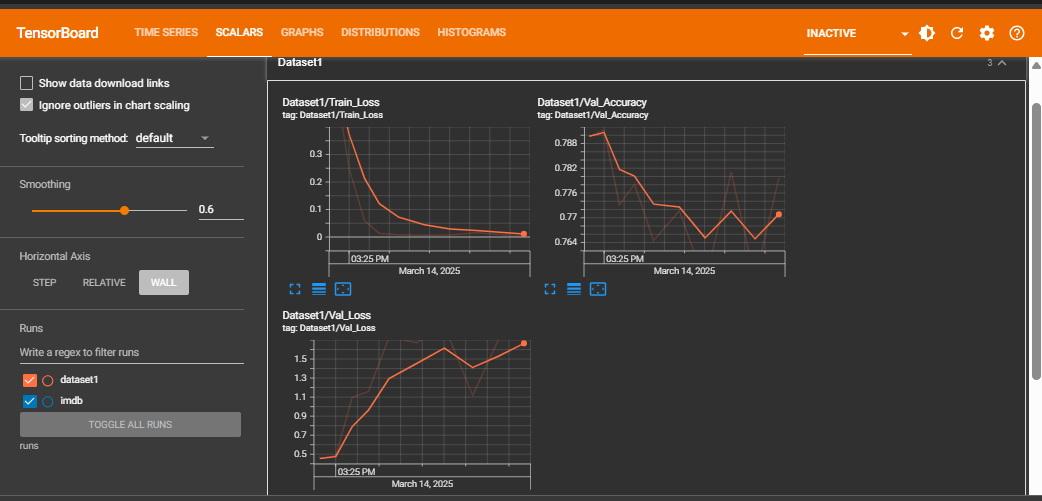
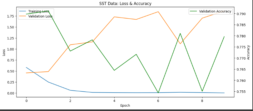
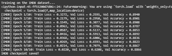
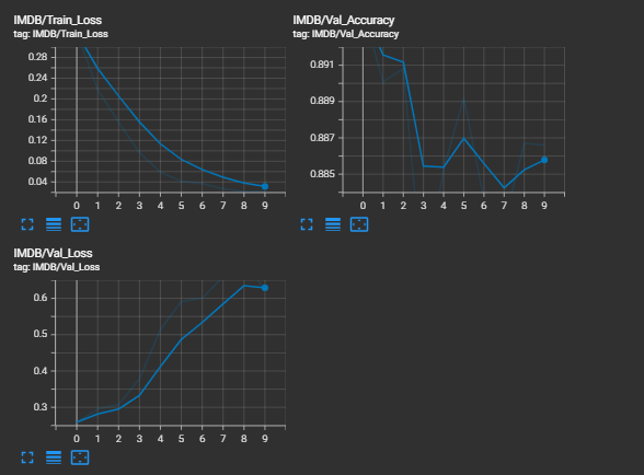
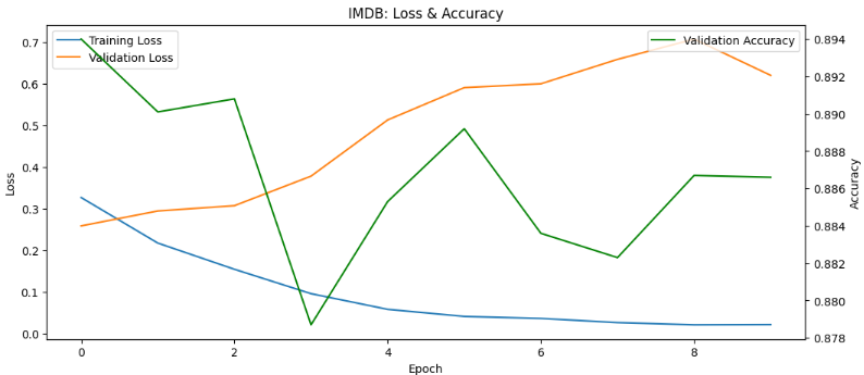
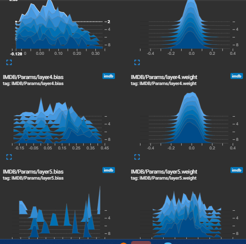
For having a personalised look at the Logged Metrics; We used TensorBoard dashboard which gives us personalised view for the same. We also used Matplotlib to plot them together
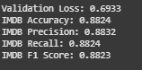
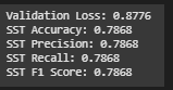
To get a better analysis we make a table which compare the evaluation results of both
| Metric | IMDB Dataset | SST Dataset |
|---|---|---|
| Validation Loss | 0.6208 | 0.8776 |
| Accuracy | 0.8866 | 0.7868 |
| Precision | 0.8867 | 0.7868 |
| Recall | 0.8866 | 0.7869 |
| F1 Score | 0.8866 | 0.7868 |
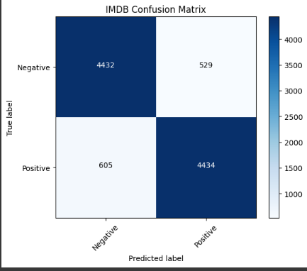
These confusion Matrices help us to visualize that how the models were accurate in predicting the sentences properly

Although we got all the required curves in TensorBoard Implementation and Also Matplotlib we make two more graphs to Analyze the Training and Validation Losses
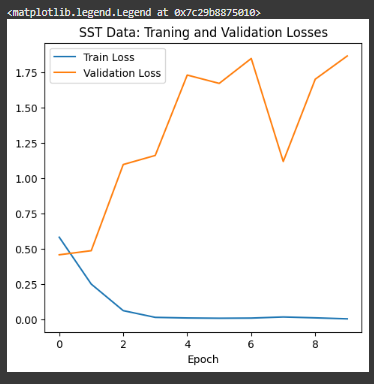
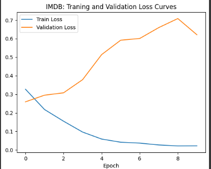
These histograms which we get from the TensorBoard Implementation for IMDB help us to analyze the cost function through the weight and biases distributions for all layers

In this assignment we observed and learnt lot of things. In the Accuracy and Losses section we observe that generally the training loss decreases over the time howver the validation loss shows some fluctuations trying to stabilise during the model training. The Validation Accuracy tries to increase itselves over the time however we get the best possible in between only. Like in the BOW case we got our best model at the second epoch only...
However considering all the parameters we can say the model is trying to get good with the epochs. When we use the checkpoint from Dataset 1 to the IMDB one; we observe a sudden increase in accuracy from around 78% to 89%, which is a good sign...
The final model gives the precision of 88.67% which shows its precision. Also the Recall and F1-Score of 88.66% suggests that model can predict true-positives and false-negatives very well compared to the 78.7% from the BOW Implementation. Again the validation loss decreased from 0.9 to 0.7 which is good mark. We are happy that we could complete the assignment and get good learnings from it.